
Star Schema Explained: A Software Engineer's Guide to Data Modeling
I am a front-end mobile and web developer. I am an AWS Community Developer. Just a guy Sharing things
Most software engineers learn data modeling in the context of application databases. You normalize tables, remove duplicate data, enforce foreign keys, and let your ORM handle the rest. That approach works well for a checkout flow or a user profile page. Then someone from the business team asks for a dashboard showing monthly revenue by product category, region, and customer segment over the last three years. You write the query against the production database, it joins nine tables, runs for forty seconds, and slows down the application while it runs.
That problem is exactly what the star schema was designed to solve. The star schema is the most widely used way to model data for analytics, and it sits underneath most data warehouses, business intelligence (BI) dashboards, and reporting tools in use today. This guide explains what a star schema is, how its parts fit together, how to design and query one, where it falls short, and how it compares to the alternatives. By the end, you should be able to look at a business question and sketch a star schema that answers it.
Overview
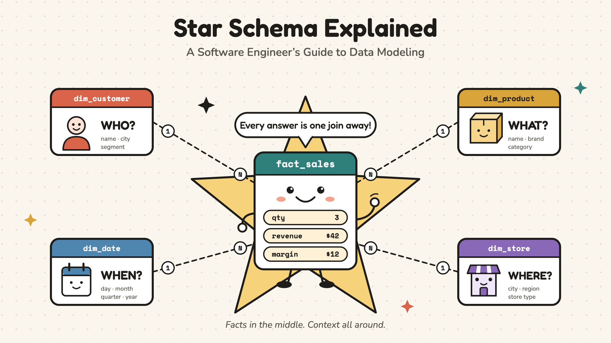
A star schema organizes data for analysis rather than for transactions. It places one large central table, called a fact table, in the middle of the model. The fact table records measurable business events such as sales, payments, or page views. Around it sit several smaller tables, called dimension tables, which describe the context of each event: who was involved, what was involved, where it happened, and when.
The design is intentionally denormalized. Instead of splitting descriptive data across many related tables, each dimension keeps its attributes together in one wide table. As a result, any analytical query can reach the context it needs with a single join from the fact table to a dimension. Fewer joins mean simpler SQL, faster queries, and a model that analysts and BI tools can understand without a map.
Why software engineers need a different model
To understand why the star schema exists, it helps to compare the two kinds of workloads that databases handle.
Application databases run what is called Online Transaction Processing (OLTP). These systems process a high volume of small, fast operations: inserting an order, updating an address, reading a single user record. Normalization, usually to third normal form (3NF), suits this workload because each fact is stored exactly once. When a customer changes their email, you update one row, and every part of the application sees the change. Data integrity is protected, and writes stay cheap.
Analytical systems run what is called Online Analytical Processing (OLAP). Here the workload is almost the opposite. Queries are few but heavy. They scan millions or billions of rows, group them, and aggregate them. Data is typically loaded in batches rather than updated one row at a time. In this world, the cost that matters most is the cost of reading and joining, not the cost of writing.
A normalized schema that serves OLTP well becomes a burden under OLAP. A question like "What was revenue by product category per region last quarter?" might need to walk from orders to order items, to products, to subcategories, to categories, then from orders to customers, to addresses, to cities, and finally to regions. Each join adds execution cost and gives the person writing the query another chance to make a mistake. The star schema flattens those paths so that every descriptive attribute sits one join away from the numbers.
| Characteristic | OLTP (application database) | OLAP (star schema) |
|---|---|---|
| Primary workload | Many small reads and writes | Few large reads and aggregations |
| Modeling style | Normalized (3NF) | Denormalized dimensions |
| Typical query | Fetch or update one record | Summarize millions of records |
| Data loading | Continuous, row by row | Batches or micro-batches |
| Optimized for | Integrity and write speed | Read speed and simplicity |
What is a star schema?
A star schema is a way of structuring tables in a data warehouse or data mart so that large volumes of data can be queried quickly and intuitively. The name comes from how the model looks when you draw it. The fact table sits in the center, and each dimension table connects directly to it, radiating outward like the points of a star.
A helpful way to picture this is a store receipt. The receipt records something that happened, along with numbers you can add up: the quantity of each item, the price, the discount, and the total. That is the fact. Everything printed around those numbers, such as the store location, the date and time, the cashier, and the product names, is context. In a star schema, the numbers live in the fact table, and the context lives in the dimensions.
The defining feature is that every dimension connects to the fact table in a single hop. Dimensions do not connect to each other. This simple, predictable shape is what makes star schemas fast to query and easy to reason about.
Components of a star schema
A star schema has two kinds of tables, and a set of keys that ties them together. Understanding each piece, and a few supporting concepts, is essential before you design one.
Fact tables
The fact table is the core of the model. Each row represents a business event or measurement, and each numeric column holds a value you want to analyze, such as revenue, quantity, cost, or duration. These numeric columns are called measures. Fact tables tend to be very long, often holding millions or billions of rows, but relatively narrow, since most columns are either measures or foreign keys pointing to dimensions.
Fact tables generally come in three forms. A transaction fact table stores one row per event, such as one row for each line on a sales order. A periodic snapshot fact table captures the state of something at regular intervals, such as the balance of every bank account at the end of each day. An accumulating snapshot fact table tracks a process with a defined beginning and end, such as an order moving from placed to paid to shipped to delivered, and updates a single row as each milestone is reached. There is also a special case called a factless fact table, which records that an event occurred without any numeric measure, such as a student attending a class.
Not every measure behaves the same way when aggregated, and this matters for correctness. Additive measures, like revenue or quantity, can be summed across every dimension. Semi-additive measures, like an account balance or inventory level, can be summed across some dimensions (for example, across accounts) but not across time, because adding Monday's balance to Tuesday's balance produces a meaningless number. Non-additive measures, like percentages or ratios, should not be summed at all. The usual approach is to store the underlying components, such as the numerator and denominator, and compute the ratio at query time.
Dimension tables
Dimension tables hold the descriptive attributes that give facts their meaning. A product dimension might contain the product name, brand, category, subcategory, color, and size. A customer dimension might contain name, city, country, and customer segment. These attributes are what users filter by, group by, and label their charts with.
Compared to fact tables, dimension tables have far fewer rows but often many more columns. They are deliberately denormalized. In an application database, category might be its own table referenced by a foreign key. In a star schema, the category name is stored directly in the product dimension, even though that means the same category name repeats across many rows. This repetition is the price paid for avoiding extra joins.
The date dimension deserves special mention because nearly every star schema has one. Rather than relying on a raw timestamp column, a date dimension stores one row per calendar day with pre-computed attributes such as day of week, month name, fiscal quarter, holiday flags, and whether the day is a weekend. This lets analysts write WHERE is_holiday = TRUE or group by fiscal quarter without writing date logic in every query, and it guarantees that every report defines those periods the same way.
Primary keys, foreign keys, and surrogate keys
Keys are the mechanism that connects the tables. Each dimension table has a primary key that uniquely identifies each row. The fact table holds a foreign key column for every dimension it references, and each of those columns points to a dimension's primary key. The fact table's own uniqueness is often defined by a combination of these foreign keys, sometimes together with an identifier such as an order number.
Star schemas usually use surrogate keys for dimensions. A surrogate key is a simple integer, or sometimes a hash, generated by the warehouse and carrying no business meaning. The original identifier from the source system, called the natural key or business key, is still stored in the dimension as an ordinary column. Engineers sometimes question this, since the application already has a perfectly good customer_id. There are several strong reasons for the extra key. Surrogate keys insulate the warehouse from changes in source systems, allow data from multiple systems with overlapping IDs to coexist, make joins on compact integers efficient, and, most importantly, make it possible to keep several historical versions of the same customer or product, which is covered later under slowly changing dimensions.
Relationships between tables
The relationships in a star schema follow two strict rules. First, every relationship between a dimension and the fact table is one-to-many: one customer appears in many sales, and one product appears in many sales. The dimension is always the "one" side, and the fact table is always the "many" side. Second, every dimension connects only to the fact table. Dimensions do not reference each other, which ensures that the path from any fact to any attribute is always exactly one join long.
Supporting concepts worth knowing
A few additional patterns appear in almost every real-world star schema. A degenerate dimension is an identifier, such as an order or invoice number, that is stored directly in the fact table because it has no other attributes worth putting in its own table. A role-playing dimension is a single dimension used several times in one fact table under different roles; an orders fact table might reference the date dimension three times, as order date, ship date, and delivery date. A junk dimension gathers miscellaneous low-cardinality flags, such as "is gift wrapped" or "payment method," into one small table instead of cluttering the fact table. Finally, a conformed dimension is a dimension that is shared, with identical meaning, across multiple fact tables, which allows a company to compare sales, returns, and marketing spend using the same definition of "customer" or "product."
The most important decision: grain
Before choosing any columns, you must declare the grain of the fact table, which is a precise statement of what a single row represents. "One row per order line item" is a grain. "One row per order" is a different grain. "One row per product per store per day" is another.
Grain matters because it determines which questions the table can answer and which dimensions can attach to it. If the fact table is stored at the order level, you cannot analyze revenue by product, because a single order contains many products. If it is stored at the order line level, you can analyze by product and still roll up to the order level when needed. The general guidance from dimensional modeling practice is to store facts at the most detailed, or atomic, grain available, since you can always aggregate detail upward but can never recover detail you did not keep.
The most common and damaging mistake in fact table design is mixing grains in one table, such as storing order-level shipping charges on every line-item row. When users sum that column, the shipping charge is counted once per line, and the totals come out wrong in a way that is easy to miss. Declaring the grain explicitly, and writing it in the table's documentation, prevents this.
A star schema example: retail sales
Consider an online retailer that wants to analyze its sales. The business process is order fulfillment, and the grain is one row per product per order, meaning one row for each line item. The model has one fact table and four dimensions.
-- Date dimension: one row per calendar day
CREATE TABLE dim_date (
    date_key        INT PRIMARY KEY,      -- e.g. 20250315
    full_date       DATE NOT NULL,
    day_of_week     VARCHAR(10),
    day_of_month    INT,
    month_number    INT,
    month_name      VARCHAR(10),
    quarter         INT,
    year            INT,
    is_weekend      BOOLEAN,
    is_holiday      BOOLEAN
);

-- Customer dimension, with history tracking columns
CREATE TABLE dim_customer (
    customer_key    INT PRIMARY KEY,      -- surrogate key
    customer_id     VARCHAR(50),          -- natural key from the app
    full_name       VARCHAR(200),
    email           VARCHAR(200),
    city            VARCHAR(100),
    country         VARCHAR(100),
    segment         VARCHAR(50),          -- e.g. 'Retail', 'Wholesale'
    valid_from      DATE,
    valid_to        DATE,
    is_current      BOOLEAN
);

-- Product dimension, denormalized
CREATE TABLE dim_product (
    product_key     INT PRIMARY KEY,
    product_id      VARCHAR(50),
    product_name    VARCHAR(200),
    brand           VARCHAR(100),
    category        VARCHAR(100),         -- stored inline, not in a separate table
    subcategory     VARCHAR(100),
    list_price      DECIMAL(10,2)
);

-- Store (or sales channel) dimension
CREATE TABLE dim_store (
    store_key       INT PRIMARY KEY,
    store_id        VARCHAR(50),
    store_name      VARCHAR(200),
    city            VARCHAR(100),
    region          VARCHAR(100),
    country         VARCHAR(100),
    store_type      VARCHAR(50)           -- e.g. 'Online', 'Flagship'
);

-- Fact table: one row per order line item
CREATE TABLE fact_sales (
    date_key        INT REFERENCES dim_date(date_key),
    customer_key    INT REFERENCES dim_customer(customer_key),
    product_key     INT REFERENCES dim_product(product_key),
    store_key       INT REFERENCES dim_store(store_key),
    order_number    VARCHAR(50),          -- degenerate dimension
    line_number     INT,
    quantity        INT,
    unit_price      DECIMAL(10,2),
    discount_amount DECIMAL(10,2),
    net_revenue     DECIMAL(12,2),
    cost_amount     DECIMAL(12,2),
    PRIMARY KEY (order_number, line_number)
);
Notice what the fact table contains: foreign keys, a degenerate order number, and numbers. It contains no product names, no customer emails, and no region labels. All descriptive text lives in the dimensions.
Querying the star schema
Suppose a manager asks for monthly net revenue and gross margin by product category for the East Africa region in 2025. Against the star schema, the query reads almost like the question itself:
SELECT
    d.year,
    d.month_name,
    p.category,
    SUM(f.net_revenue)                  AS revenue,
    SUM(f.net_revenue - f.cost_amount)  AS gross_margin
FROM fact_sales f
JOIN dim_date    d ON f.date_key    = d.date_key
JOIN dim_product p ON f.product_key = p.product_key
JOIN dim_store   s ON f.store_key   = s.store_key
WHERE d.year = 2025
  AND s.region = 'East Africa'
GROUP BY d.year, d.month_number, d.month_name, p.category
ORDER BY d.month_number, revenue DESC;
Every join follows the same pattern: fact table to dimension, on a single integer key. There is no need to know how the application stores categories or addresses. The equivalent query against a normalized application schema would typically chain through order items, products, subcategories, categories, orders, customers or stores, addresses, cities, and regions, and it would need date functions to derive months. The star schema version is shorter, easier to review, and much easier for a database engine to optimize.
This pattern is sometimes described as "slicing and dicing": take a measure, filter it by some dimension attributes, and group it by others. BI tools such as Power BI, Tableau, and Looker are built around exactly this interaction, which is why star schemas work so smoothly with them.
Handling change: slowly changing dimensions
Dimension data changes over time. Customers move, products get recategorized, and stores are reassigned to new regions. The question is what should happen to historical reports when that happens. If a customer moved from Nairobi to Mombasa in June, should their January purchases be reported under Nairobi or Mombasa? Dimensional modeling answers this with techniques called slowly changing dimensions (SCDs), and engineers will recognize them as a form of data versioning.
Type 1 simply overwrites the old value. The customer's city becomes Mombasa, and all past sales now appear under Mombasa. This is easy to implement and appropriate for corrections, such as fixing a misspelled name, but it rewrites history.
Type 2 preserves history by inserting a new row whenever a tracked attribute changes. The customer keeps the same natural key but receives a new surrogate key. The old row is closed by setting its valid_to date and marking is_current as false, while the new row starts with a fresh valid_from date. Sales recorded before the move point to the old surrogate key, and sales after the move point to the new one, so every report reflects where the customer lived at the time of each purchase. This is the most common approach for attributes that matter analytically, and it is the main reason surrogate keys are so important.
Type 3 adds a column to hold the previous value, such as previous_city, allowing limited comparison between the current and prior state without keeping full history. It is used less often.
In practice, many teams mix these approaches within one dimension, applying Type 1 to attributes where history is irrelevant and Type 2 to attributes where it matters. Modern tools make Type 2 easier to manage; dbt, for instance, provides a snapshot feature that detects changes and maintains the validity columns automatically.
Advantages of a star schema
The star schema's popularity comes from a set of practical benefits, all of which follow from its simple, read-optimized shape.
Simplicity and ease of understanding
The separation between facts and dimensions maps naturally to how people think about business questions. Analysts, product managers, and engineers can look at the model and understand it quickly, because every question follows the same pattern of measuring something and describing it by some context. That clarity reduces errors, shortens onboarding for new team members, and makes self-service analytics realistic for non-technical users.
Faster query performance
Because dimension attributes are stored together, queries need far fewer joins than they would against a normalized model. Joining a large fact table to small dimension tables on integer keys is a pattern that database optimizers handle very efficiently. Many engines apply specific techniques for it, such as building hash tables from the small dimensions, pushing filters down, and skipping large portions of the fact table that cannot match. The result is consistently fast response times, even over very large datasets.
Strong compatibility with BI and OLAP tools
BI platforms and semantic layers are designed around measures and dimensions. When the underlying data is already organized that way, these tools can generate efficient SQL, present intuitive field lists to users, and aggregate correctly with little configuration. Power BI in particular is well known for performing best, and producing the most reliable results, when its data model follows a star shape.
Consistent, reusable definitions
When dimensions are conformed and shared across fact tables, everyone in the organization works from the same definitions of customer, product, and time. This reduces the familiar problem of two dashboards showing two different revenue numbers for the same period.
Predictable, maintainable pipelines
A star schema gives data pipelines a clear target. Dimensions are loaded first, facts are loaded second with lookups to dimension keys, and every table has a well-defined purpose. This structure makes transformation code easier to test, document, and extend.
Disadvantages of a star schema
The star schema is a trade-off, and it is worth understanding what you give up.
Data redundancy
Denormalized dimensions repeat values. A category name or region label may appear thousands of times in a dimension table. This uses more storage than a normalized design. In modern columnar warehouses, compression reduces the impact considerably, since repeated values compress very well, but the redundancy still exists in the logical model.
More complex loading and integrity management
Because data is duplicated and history may be tracked, loading processes must be designed carefully. Pipelines must look up the correct surrogate key for each fact, handle late-arriving data, manage Type 2 changes, and avoid orphaned records. Integrity that a normalized database would enforce automatically becomes the responsibility of the pipeline and its tests.
Poor fit for write-heavy workloads
Star schemas are built for reading. Frequent single-row updates, inserts, and deletes are awkward and slow compared to a normalized transactional database. A star schema should never replace your application database; it should sit downstream of it.
Rigidity around grain and scope
A star schema is designed around specific business processes and a chosen grain. If requirements change dramatically, such as needing a finer grain than was stored, the model may need to be rebuilt. Careful upfront design and storing data at the atomic grain reduce this risk.
Star schema vs. snowflake schema
The snowflake schema is the closest alternative to the star schema, and the difference between them comes down to how dimensions are structured.
Structure and normalization
In a star schema, each dimension is a single, wide, denormalized table connected directly to the fact table. In a snowflake schema, dimensions are normalized into several related tables. For example, the product dimension might reference a separate subcategory table, which in turn references a category table. Drawn out, these branching dimensions resemble the arms of a snowflake. (The schema's name is unrelated to the Snowflake data platform, which supports both designs.)
Query performance
Star schemas usually query faster because every attribute is one join away. Snowflake schemas require additional joins to reach attributes stored in sub-dimension tables, which adds complexity to the SQL and more work for the query engine.
Storage and maintenance
Snowflake schemas store less redundant data, and changes to a shared attribute, such as renaming a category, happen in one place. Star schemas trade that efficiency for speed and simplicity. With modern storage costs and columnar compression, the storage savings of snowflaking are rarely decisive on their own.
Choosing between them
A star schema is generally the better default for BI dashboards, ad hoc analysis, and any environment where ease of use matters. A snowflake schema can make sense when a dimension is very large with deep hierarchies, when certain sub-dimensions are maintained by different teams, or when strict avoidance of redundancy is a priority. Many real-world warehouses use a hybrid, keeping most dimensions flat and normalizing only where there is a clear reason.
| Aspect | Star schema | Snowflake schema |
|---|---|---|
| Dimension structure | Single denormalized table | Normalized into multiple tables |
| Joins per attribute | One | One or more |
| Query speed | Generally faster | Generally slower |
| Storage redundancy | Higher | Lower |
| Ease of use | Simpler | More complex |
| Best suited for | BI, dashboards, ad hoc queries | Deep hierarchies, strict normalization needs |
Other alternatives worth knowing
The star schema is not the only analytical model in use, and engineers will encounter a few others.
One Big Table (OBT) takes denormalization to its limit by joining facts and all dimension attributes into a single wide table. Columnar warehouses such as BigQuery and Snowflake handle wide tables well, so OBT can be convenient for specific use cases like feeding a single dashboard or a machine learning feature pipeline. Its drawbacks are that dimension changes require rewriting large amounts of data and that definitions are harder to keep consistent across many wide tables. A common pattern is to build a star schema as the governed core and generate OBTs from it where needed.
Data Vault is a modeling approach designed for integrating many source systems while preserving full history and auditability. It uses hubs, links, and satellites, and it is typically used in the raw or integration layer of large enterprise warehouses. Star schemas are often built on top of a Data Vault layer for reporting.
Third normal form (3NF) remains the right choice for application databases and some enterprise integration layers, but it is rarely the best structure for end-user analytics.
Star schemas in the modern data stack
It is reasonable to ask whether star schemas still matter now that cloud warehouses can scan enormous tables quickly and cheaply. The answer is yes, though the reasons have shifted somewhat. Raw performance is less of a constraint than it once was, but clarity, consistency, and governance matter more than ever as more people and tools query the same data.
In a typical modern setup, data is extracted from application databases, SaaS tools, and event streams, then loaded into a warehouse such as Snowflake, BigQuery, Redshift, or Databricks. Transformation happens inside the warehouse, often using dbt, following an extract, load, transform (ELT) pattern. Teams usually organize their transformations in layers: a staging layer that cleans and renames raw source data, an intermediate layer that applies business logic, and a final marts layer where facts and dimensions live. Naming conventions such as fct_ and dim_ prefixes make the star schema visible directly in the project structure.
Physical optimization also looks different in cloud warehouses. Traditional databases relied on indexes, including bitmap indexes on dimension keys. Many cloud warehouses do not use conventional indexes at all; instead, they rely on columnar storage, partitioning, clustering keys, and metadata that allows the engine to skip data that cannot match a filter. Partitioning or clustering the fact table by date is one of the most effective optimizations available, since most analytical queries filter on time.
Designing and implementing a star schema
Designing a star schema is a structured process. The widely used method from Ralph Kimball's dimensional modeling approach breaks it into four steps, followed by the practical work of building and loading the tables.
1. Choose the business process
Start with a specific business activity that generates measurable events, such as taking orders, processing payments, handling support tickets, or recording user sessions. Model processes, not departments. A "sales department" is not a process; "order fulfillment" is.
2. Declare the grain
State precisely what one row in the fact table represents, and write it down. Prefer the most atomic grain available from the source systems. Every later decision must be consistent with this statement.
3. Identify the dimensions
Ask how people describe each event. Who was the customer? What product was involved? Where did it happen? When did it happen? Through which channel? Each of these answers suggests a dimension. Only include dimensions that have a single value for each row at the declared grain.
4. Identify the facts
Determine which numeric measures are true at the declared grain, such as quantity, amount, and cost. Classify each measure as additive, semi-additive, or non-additive so that reports aggregate it correctly. Avoid storing values that belong to a different grain.
5. Define keys and physical structure
Create surrogate keys for each dimension and keep the natural keys as attributes. Decide which attributes need Type 1 or Type 2 change handling. Add an "Unknown" or "Not applicable" row to each dimension, usually with a key such as -1, so that facts with missing references still join correctly instead of disappearing from reports or producing null groupings. Choose partitioning or clustering for the fact table based on common filters.
6. Build and load the data
Load dimensions first, applying change handling as needed. Then load facts, looking up the correct surrogate key for each record. Add data quality tests to check that keys are unique, foreign keys resolve to real dimension rows, and totals reconcile with the source systems. As more fact tables are added, a bus matrix, a simple grid showing which dimensions each business process uses, helps keep dimensions conformed across the warehouse.
Common mistakes to avoid
Several pitfalls appear repeatedly in star schema projects. Mixing grains in a single fact table leads to double-counted totals. Storing descriptive text in the fact table bloats it and undermines the model's structure. Using natural keys from the application instead of surrogate keys makes history tracking and multi-source integration difficult. Skipping the date dimension forces every analyst to reimplement calendar logic, often inconsistently. Over-snowflaking dimensions adds joins without meaningful benefit. Summing semi-additive measures across time produces numbers that look plausible but are wrong. Finally, leaving foreign keys null instead of pointing to an "Unknown" row causes records to silently drop out of inner joins.
When to use a star schema
A star schema is the right choice in many analytical situations. It fits best when read performance and fast response times are a priority, especially for dashboards that many people use throughout the day. It is ideal when the data will be consumed through BI tools or semantic layers that think in terms of measures and dimensions. It suits organizations that want non-technical users to explore data on their own, since the model is easy to learn. It is valuable when consistent aggregation and shared definitions across teams are important. And it works well when data arrives in batches or micro-batches and the focus is on analyzing historical trends.
When not to use one
A star schema is not the right tool for everything. It should not serve as the database behind a transactional application, where normalized designs remain the correct choice. It adds unnecessary ceremony for very small datasets or one-off analyses, where a simple query or spreadsheet is enough. It is a poor match for highly unstructured or rapidly changing data whose shape is not yet understood. It can also be less suitable for workloads that require sub-second updates to individual records, which are better served by operational databases or specialized real-time systems.
Conclusion
The star schema remains the foundation of analytical data modeling because it aligns the structure of data with the way people ask questions about a business. A central fact table captures what happened, surrounding dimensions explain the context, and every attribute is one join away from the numbers. For software engineers, the key mental shift is moving from a model optimized for safe, efficient writes to one optimized for fast, understandable reads.